We call IXP Manager’s statistics and graphing architecture Grapher. It’s a backend agnostic way to collect and present data. Out of the box, we support MRTG for standard interface graphs, sflow for peer to peer and per-protocol graphs, and Smokeping for latency/packet loss graphs. You can see some of this in action on INEX’s public statistics section.
Internet Exchange Points (IXPs) play a significant role in national internet infrastructures and IXP Manager is used in nearly 100 of these IXPs worldwide. In the last couple weeks we have got a number of queries from those IXPs asking for suggestions on how they can extract traffic data to address queries from their national Governments, regulators, media and members. We just published our own analysis of this for traffic over INEX here.
Grapher has a basic API interface (documented here) which we use to help those IXP Manager users address the queries they are getting. What we have provided to date are mostly quick rough-and-ready solutions but we will pull all these together over the weeks (and months) to come to see which of them might be useful permanent features in IXP Manager.
How to Use These Examples
The code snippets below are expected to be placed in a PHP file in the base directory of your IXP Manager installation (e.g. /srv/ixpmanager) and executed on the command line (e.g. php myscript.php).
Each of these scripts need the following header which is not included below for brevity:
<?php

require 'vendor/autoload.php';

use Carbon\Carbon;

$data = json_decode( file_get_contents(
    'https://www.inex.ie/ixp/grapher/ixp?period=year&type=log&category=bits'
) );
We’ve placed a working API endpoint for INEX above – change this for your own IXP / scenario.
Data Volume Growth
An IXP was asked by their largest national newspaper to provide daily statistics of traffic growth due to COVID-19. For historical reasons linked to MRTG graph images, the periods in IXP Manager for this data is such that: day is last 33.3 hours; week is last 8.33 days; month is last 33.33 days; and year is last 366 days.
This is fine within IXP Manager when comparing averages and maximums as we are always comparing like with like. But if we’re looking to sum up the data exchanged in a proper 24hr day then we need to process this differently. For that we use the following loop:
$start = new Carbon('2020-01-01 00:00:00');
$bits = 0;
$last = $data[0][0];
$startu = $start->format('U');
$end = $start->copy()->addDay()->format('U');

foreach( $data as $d ) {
  // if the row is before our start time, skip
  if( $d[0] < $startu ) { $last = $d[0]; continue; }

  if( $d[0] > $end ) {
    // if the row is for the next day break out and print the data
    echo $start->format('Y-m-d') . ','
        . $bits/8 / 1024/1024/1024/1024 . "\n";

    // and reset for next day
    $bits  = $d[1] * ($d[0] - $last);
    $startu = $start->addDay()->format('U');
    $end    = $start->copy()->addDay()->format('U');
  } else {
    $bits += $d[1] * ($d[0] - $last);
  }

  $last = $d[0];
}
The output is comma-separated (CSV) with the date and data volume exchanged in that 24 hour period (in TBs via 8/1024/1024/1024/1024). This can, for example, be pasted into Excel to create a simple graph:
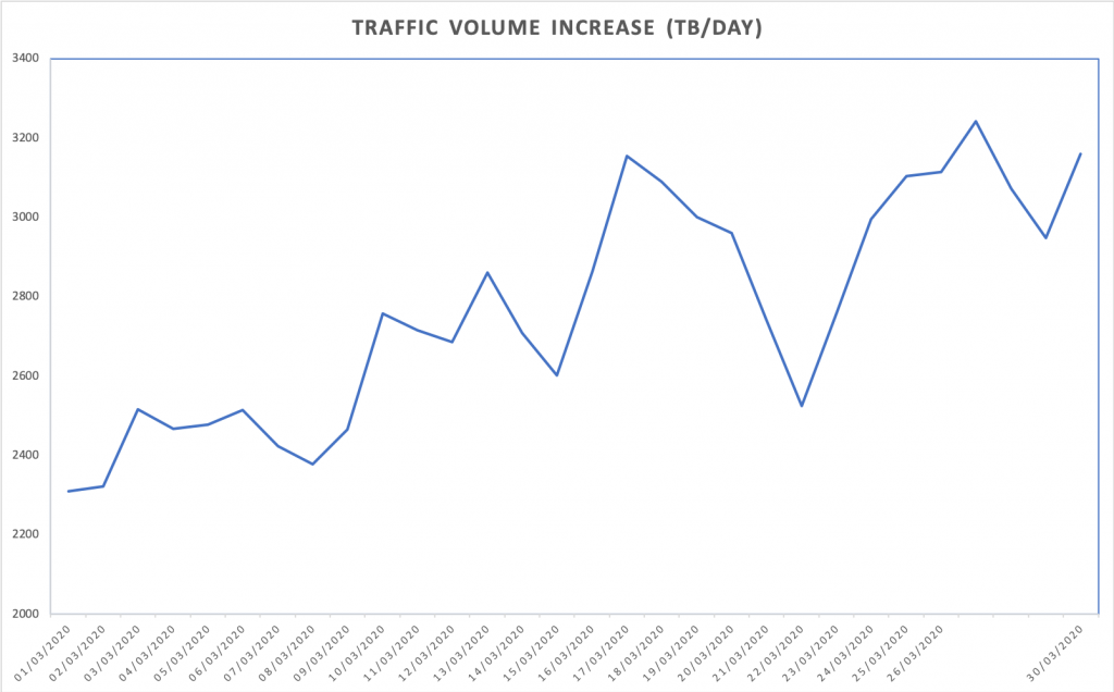
The elements of the $d[] array mirror what you would expect to find in a MRTG log file (but the data unit represents the API request – e.g. bits/sec, pkts/sec, etc.):
d[0]– the UNIX timestamp of the data sample.$d[1]and$d[2]– the average incoming and outgoing transfer rate in bits per second. This is valid for the time between the$d[0]value of the current entry and the$d[0]value of the previous entry. For an IXP where traffic is exchanged, we expect to see$d[1]roughly the same as$d[2].$d[3]and$d[4]– the maximum incoming and outgoing transfer rate in bits per second for the current interval. This is calculated from all the updates which have occured in the current interval. If the current interval is 1 hour, and updates have occured every 5 minutes, it will be the biggest 5 minute transfer rate seen during the hour.
Traffic Peaks
The above snippet uses the average traffic values and the time between samples to calculate the overall volume of traffic exchanged. If you just want to know the traffic peaks in bits/sec on a daily basis, you can do something like this:
$daymax = 0;
$day    = null;

foreach( $data as $d ) {

    $c = ( new Carbon($d[0]) )->format('Y-m-d');

    if( $c !== $day ) {
        if( $day !== null ) {
            echo $day . ',' . $daymax / 1000/1000/1000 . "\n";
        }
        $day = $c;
        $daymax = $d[3];
    } else if( $d[3] > $daymax ) {
        $daymax = $d[3];
    }
}
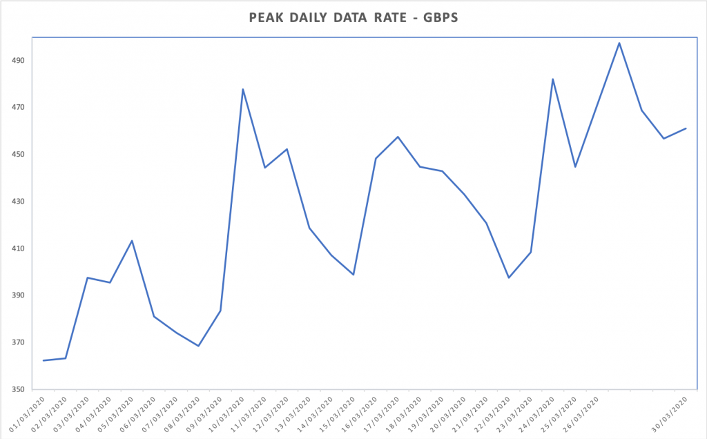
The output is comma-separated (CSV) with the date and data volume exchanged in that 24 hour period (in Gbps via 1000/1000/1000). This can also be pasted into Excel to create a simple graph:
Import to Carbon / Graphite / Grafana
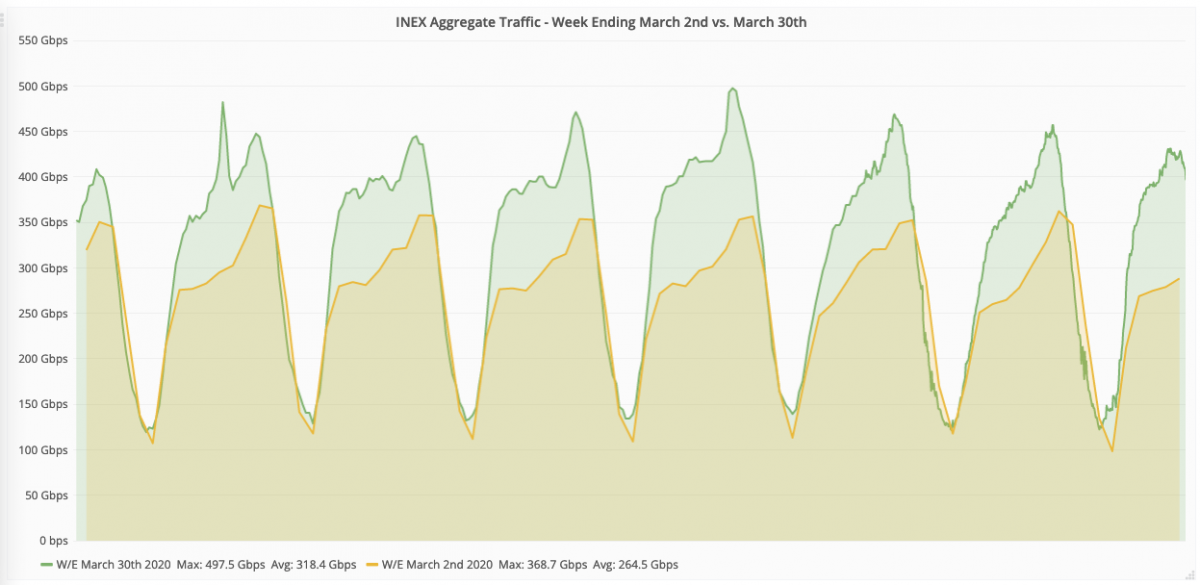
Something that is on our development list for IXP Manager is to integrate Graphite as a Grapher backend. Using this stack, we could create much more visually appealing graphs as well as time-shift comparisons. In fact this is how we created the graphs for this article on INEX’s website which includes graphs such as:
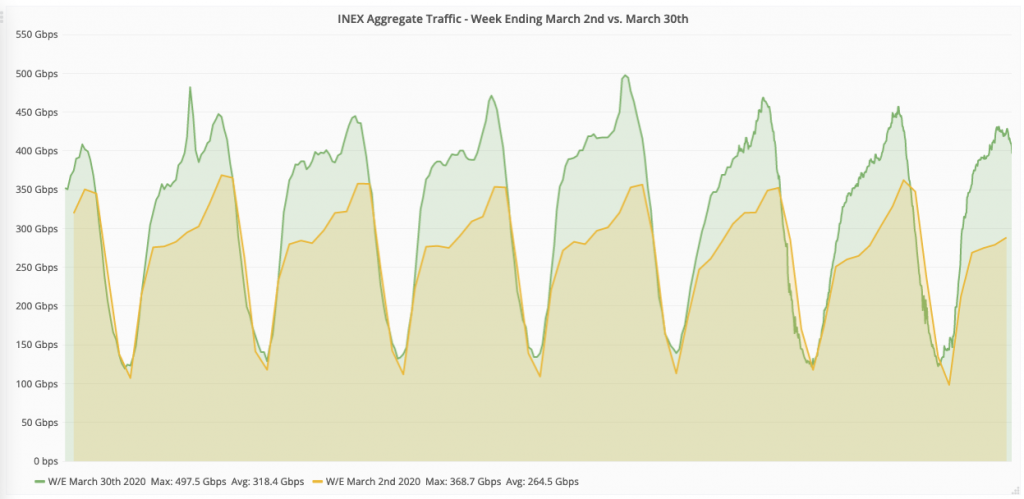
To create this, we need to get the data into Carbon (Graphite’s time-series database). Carbon accepts data via UDP so we used a script of the form:
foreach( $data as $d ) {
    echo "echo \"inex.ixp.run1 " . $d[1] . " " . $d[0]
        . "\" | nc <carbon-ip-address> 2003\n";
}
This will output lines like the following which can be piped to sh:
echo "inex.ixp.run1 387495973600 1585649700" | nc -u 192.0.2.23 2003
The Carbon / Graphite / Grafana stack is quite complex so unless you are familiar with it, this option for graphing could prove difficult. To get up and running quickly, we used the docker-grafana-graphite Docker image. Beware that the default graphite/storage-schemas.conf in this image limits data retention to only 7 days.